OpenMETA Vahana Case Study - Part I
/An OpenMETA model for the conceptual design of an electric single-passenger aircraft based on A3's Vahana Configuration Trade Study
Summary
Using A3's publicly-released source code, we built OpenMETA models of the Vahana tilt-wing multirotor aircraft and a generic electric helicopter.
Then, using the OpenMETA toolset, we performed a multidisciplinary optimization and analysis of the two models across a range of operating distances.
early conceptual sketch of Vahana tilt-wing aircraft
Source: A^3 Welcome to vahana
Our initial results replicate A3’s and suggest that an electric tilt-wing multirotor aircraft offers a significantly lower direct operating cost (DOC) over the more traditional electric helicopter design around the target operational range of 100 km.
At operating distances exceeding 35 km, the conceptual Vahana design offers a DOC reduction of up to $0.60/km (a percentage decrease of 39%) versus the electric helicopter design. Furthermore, if the models are modified to limit their fuel weights to less than one third of their maximum vehicle takeoff weights, then this DOC difference increases dramatically.
At the target operational range of 100 km, the optimized helicopter configuration has a cruise speed that is 24% greater than the optimized tilt-wing configuration's; however, when the tilt-wing model's cruise speed is adjusted to match the helicopter model, the tilt-wing configuration still offers a substantial DOC reduction when compared to the electric helicopter configuration.
Both vehicle configuration models enjoy cruise speeds well in excess of what a traditional car might expect on the interstate and share the ability to take more direct paths of travel while bypassing ground traffic gridlock. Therefore, we believe that, of the two configuration models examined, the electric tilt-wing is the best option given its lower minimum DOC at the target operating range of 100 km.
A3 Vahana Configuration Trade Study
Located in Silicon Valley, A3 is the advanced projects branch of global aerospace leader Airbus. In early 2016, A3 started work on Project Vahana, an ambitious campaign to create a low-cost, single-passenger, electric VTOL aircraft.
Project Vahana is A3’s response to growing traffic problems in large urban areas where severe congestion has become a major pain-point for commuters, businesses, and city planners.
A3 conducted a trade study using multidisciplinary design analysis and optimization (MDAO) techniques to arrive at a multi-rotor tilt-wing design for the Vahana.
In the Vahana Configuration Trade Study, A3 compared two conceptual designs - an electric, eight-fan tilt-wing and an electric helicopter - over a range of operating distances from 10 to 200 km. At each distance, a numerical optimization approach was used to minimize the direct operating costs of each vehicle model by varying key design variables: cruise speed, rotor radius, battery mass, motor mass, and maximum takeoff mass.
One of the key findings from the Vahana Configuration Trade Study was that the tilt-wing design’s superior cruise characteristics resulted in a substantial decrease in direct operating costs compared to the helicopter design at operating ranges over 70 km. This phenomena is illustrated in the image below. Consequently, A3 concluded that an eight-fan, tilt-wing configuration would best meet their conceptual design requirements for a low-cost, single-passenger, electric VTOL aircraft.
A^3 Vahana configuration trade study results
source: vahana CONFIGURATION Trade study - part ii
The Vahana Configuration Trade Study provides an excellent example of how multidisciplinary design analysis and optimization techniques (MDAO) can be used in the conceptual design of a complex system. MDAO techniques and tools allows designers to rapidly compare broad design options and quickly eliminate infeasible design paths.
In the design world, the 80-20 rule suggests that decisions made early in the design process have a much greater impact on development costs than design decisions made later on. Conceptual design choices limit future decisions and are hard to test initially. In the aerospace industry, conceptual design choices can account for more than 80% of development costs.1
MDAO tools like OpenMETA help designers to make critical design choices early in the design process through the use of multidomain models, integrated workflows, and multidisciplinary analysis - resulting in lower development costs, shorter design lifecycles, and a better end product.
Building the OpenMETA Vahana Model
In addition to publishing two blog posts explaining their Vahana
Trade Study results, A3 also made the trade study
source
code publicly available on GitHub under an MIT License. Here at
MetaMorph, we decided that the Vahana Trade Study would make
a good case study for the OpenMETA toolset. Our goals were to:
Converting A3's MATLAB Scripts to OpenMDAO Component Python Scripts
For their trade study, A3 modeled the electric tilt-wing and helicopter designs using MATLAB scripts. The structure of their code is shown in the figure below.
A^3 Vahana configuration trade study code structure
Source: METAMORPH, INC.
Instead of copying this structure exactly, we chose to restructure it to represent value flow through the model in a more linear fashion. Doing so came at a trade-off. It made tracking value flow through the model easier, but the reduced encapsulation also made some aspects of the model visually messy.
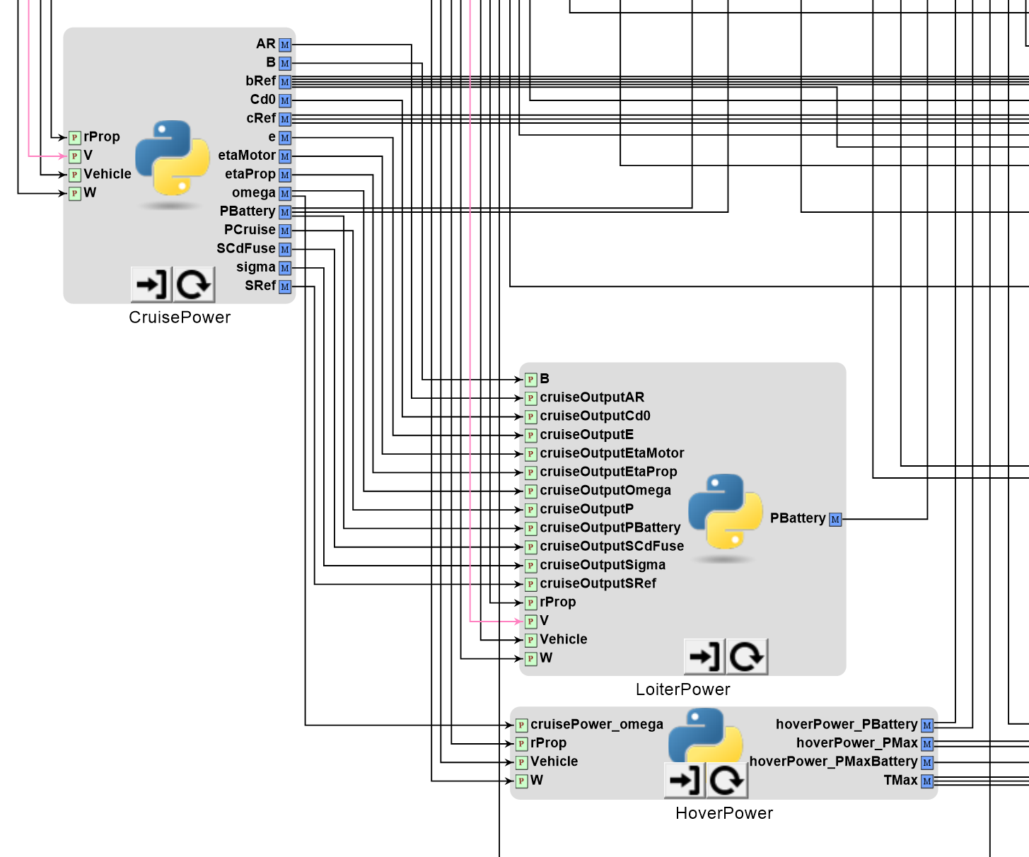
The first step in this process was to convert A3's MATLAB scripts into OpenMDAO Component Python Scripts (Python Wrapper components in OpenMETA). The Python Wrapper component allows us to define an arbitrary block of Python code (e.g.: a model, system, or calculation, with explicit inputs and outputs). This Python Wrapper component can be placed within an OpenMETA model where its inputs and outputs are exposed as ports.
For example, in the A3 trade study, the MATLAB script 'configWeight()', defined in 'configWeight.m', is called in the 'computePerformance.m' script as shown below.
% Mass estimate
mass = configWeight(vehicle,rProp,mBattery,mMoters,mtow,hoverOutput,cruiseOutput,payload);
We converted the contents of 'configWeight.m' to a Python Wrapper
component python script, 'config_weight.py.' When 'config_weight.py'
is placed within an OpenMETA Parametric Exploration Tool (PET), it
appears
as a block with input and ouput ports on the left and right side
respectively as shown below.
Note, while the MATLAB script
returned a 'mass' array and took in several other arrays as
function arguments, we chose to represent all the inputs
and outputs as scalars.
OpenMETA Vahana: configweight Python wrapper component
source: metamorph, inc.
It's worth noting that, for our purposes, the conversion from MATLAB to Python was not always exact. We had to find subsitutes for many of the built-in MATLAB functions/constructs, and as mentioned earlier, we took some liberties in recomposing parts of the model to better fit within the OpenMETA architecture.
In a similar fashion to 'configWeight.m,' all the appropriate A 3 MATLAB scripts were converted to Python Wrapper components, connected, and used as 'building blocks' to compose the larger Vahana model within the Parametric Exploration Tool canvas.


Adding an Optimization Driver
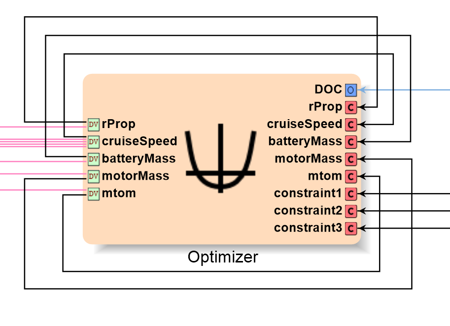
We added an Optimizer PET driver to our Vahana model and configured it to minimize direct operating cost by varying the prop radius, cruise speed, battery mass, motor mass, and maximum takeoff mass within their design ranges. We also added three optimizer constraints to the driver - one for each of the constraint components.
Setting up a Design of Experiements (DoE)
At this point, we had assembled an OpenMETA PET model of the Vahana tilt-wing configuration using Python Wrapper components, added an Optimizer driver to the PET, and made the appropriate connections. Running this PET produced identical data to the Vahana Configuration Trade Study.
The final step in building the OpenMETA Vahana model was setting up a DoE to generate independent optimized vehicle models for each of the twenty operating ranges. In OpenMETA Version 0.13.0, we introduced PET hierarchies to support DoEs, nested optimization blocks, and additional layers of encapsulation. Using these recently-added PET hierarchy changes, we placed our entire OpenMETA PET model of the Vahana tilt-wing design inside another PET containing a Parameter Study driver as shown below.
Top-level PET with parameter study driver and Vahana tilt-wing optimizer PET
source: metamorph, inc.
The Parameter Study driver in the image above varies the Range Parameter between 10 km to 200 km. Each Range value is passed into the Vahana Tilt-wing Optimizer PET (shown below) which then optimizes the direct operating cost by changing the five design variables. The direct operating costs and final design variable values are then passed back out to the top level PET where they are recorded by the Parameter Study driver.
Below is a more abstract representation of signal flow and PET hierarchy in the OpenMETA Vahana Model.
OpenMETA Vahana: PET hierarchy diagram
Source: metamorph, inc.
We also built an electric helicopter configuration PET using the same process. We could have combined the analyses for both vehicle configurations into one PET model, but for the sake of clarity, we opted to build seperate tilt-wing and helicopter PET models. Since we built the tilt-wing model out of modular Python Wrapper components, we were able to reuse large parts of it in the helicopter model with only slight changes.
Analyzing the OpenMETA Vahana Model
Direct Operating Cost Analysis
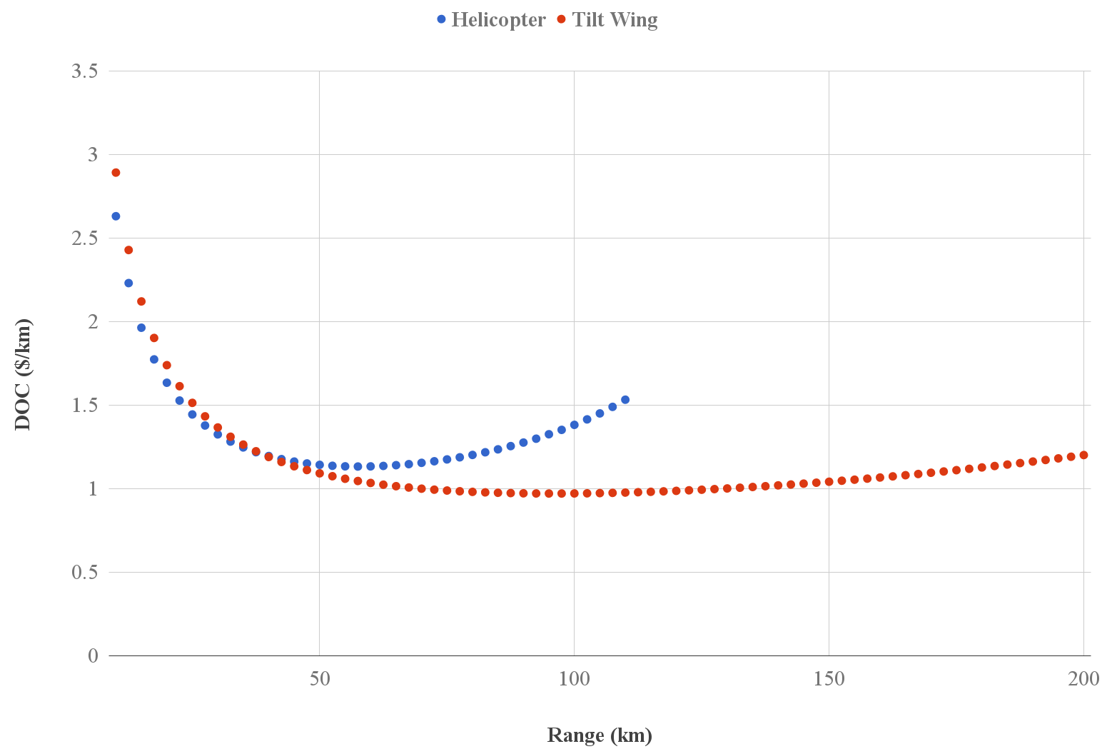
After building PET models for both the electric tilt-wing and helicopter designs, we were ready to run some analyses on the models. As shown in the graph below, our DOC vs. Range results match those obtained in the Vahana Configuration Trade Study.
OpenMETA Vahana results: DOC vs. range for tilt-wing and helicopter configurations
SOUrce: METAMORPH, INC.
As shown in the figure above,
the electric tilt-wing configuration's superior cruise efficiency gives
it an advantage at ranges exceeding about 35 km.
At Project Vahana's target operational range of 100 km, it would cost
$138 to travel in the electric helicopter but only $93 to travel in
the electric tilt-wing. At 100 km, the electric tilt-wing's DOC per km
is $0.60 (39%) less than the helicopter's.
Note: the
Helicopter data stops at 110 km because the helicopter model cannot
satisfy all four of its constraint equations at ranges past that.
The direct operating cost breakdowns for both configurations at 100 km are shown below. Values are in USD.
Direct Operating Cost Breakdown at 100 km
For both configuration models, the largest single contributer to direct operating cost is part replacement. The helicopter model's part replacement cost is nearly twice that of the tilt-wing model. Part replacement cost in both models is overwhelmingly a function of battery replacement cost. The battery lifespan is fixed at an assumed value of 2000 cycles for both configurations, so differences in battery replacement costs must result from different energy requirements.
The mass breakdowns for both configurations at 10, 50, and 100 km are shown below. Values are in kg.
Mass Breakdown at 10, 50, and 100 km
From the charts above, we can see that the helicopter configuration model's battery mass increases with operating range at a faster rate than the tilt-wing configuration model's battery mass. This is to be expected given the aerodynamic advantage the tilt-wing configuration enjoys when cruising.
Cruise Speed Analysis
Part of Project Vahana's allure is the premise of fast urban transportation. The graph below shows cruise speed vs. range for both configurations.
OpenMETA Vahana results: cruise speed vs. range for tilt-wing and helicopter configurations when optimized for DOC
Source: Metamorph, inc.
The tilt-wing model's optimum cruise speed starts out at 52.0 m/s at the 10 km operating range and decreases lineaerly to 46.4 m/s at 200 km. The helicopter model's optimum cruise speed curve is more interesting and significantly higher than the tilt- wing's. At Vahana's target operating range of 100 km, the tilt-wing model's cruise speed of 48.6 m/s is 19% slower than the helicopter model's cruise speed of 60.1 m/s.
Assuming marginal take-off and landing times, a 100 km trip in the electric tilt-wing configuration would take roughly 34.3 min, where the same 100 km trip would take about 27.7 min in the electric helicopter configuration. For reference, a car driving at 26.8 m/s (roughly 60 mph) would take 62 min to complete the 100 km trip - assuming no traffic and a direct as-the-crow-flies road.
This is an interesting result. At the Vahana's target operational range of 100 km, the tilt-wing's DOC is 39% less than the helicopter's, but the helicopter's cruise speed is 24% greater than the tilt-wing's at that range.
We wanted to see how the tilt-wing and helicopter models' costs compared at similar cruise speeds. To do this, we simply increased the minimum value for the cruise speed design variable to 60.0 m/s in the tilt-wing PET model and reran the PET. The DOC vs. Range results are shown below.
OpenMETA Vahana results: DOC vs. range for tilt-wing and helicopter configurations at similar cruise speeds
Source: Metamorph, inc.
Increasing the tilt-wing model's minimum cruise speed did not significantly affect its DOC advantage over the electric helicopter configuration.
The PET changes we made to the tilt-wing model increased its cruise speed to be comparable to the helicopter's as shown below.
OpenMETA Vahana results: cruise speed vs. range for tilt-wing and helicopter configurations when optimized for doc and tilt-wing cruise speed minimum value increased to 60 m/s
Source: Metamorph, inc.
Adding a Fuel Weight Constraint to the Model
In the original A3 blog post, Geoffrey Bower states that for most transport aircraft the maximum fuel weight is capped at roughly a third of the maximum takeoff weight.
In order to see what effect this would have on the model, we added a FuelWeightConstraint function to the OpenMETA model using a Python Wrapper component and connected it to the Optimizer driver as a constraint.
Fuel weight constraint function added as Python wrapper component
Source: metamorph, inc.
Fuel Weight constraint connected to optimizer
Source: METAMORPH, INC.
The fuel weight constraint affect on the tilt-wing PET model's DOC vs. Range curve is shown below.
OpenMETA Vahana results: DOC vs. range for tilt-wing configuration with and without fuel weight constraint
Source: METAMORPH, INC.
Adding the fuel weight constraint changes the tilt-wing configuration's DOC vs. Range curve, causing it to start rising at operating ranges of 75 km and greater. For the Vahana aircraft's target operational range of 100 km, this weight restriction translates into a $0.07 difference in DOC per km ($7 per 100 km trip).
For good measure, we also ran a simulation comparing the tilt-wing and helicopter with the added fuel weight constraint. As shown below, enforcing the constraint dramatically reduces the electric helicopter configuration's range and increases its cost, making the tilt-wing the better option.
OpenMETA Vahana results: DOC vs. range for tilt-wing and helicopter configurations with fuel weight constraint
Source: METAMORPH, INC.
OpenMETA Vahana Source Code
All the PET models as well as the source code for the PET Analysis Blocks are available on GitHub: https://github.com/metamorph-inc/openmeta-vahana
The openmeta-vahana repository README.md includes detailed instructions on how to install OpenMETA and start playing with the OpenMETA Vahana PET models. Additional information and tutorials on the OpenMETA toolset can also be found in the documentation.
In addition to the PETs covered so far, we also included a couple PETs with exposed top-level parameters (like the one shown below), so that you can see how different battery energy densities, battery life cycles, electricity costs, production volumes, etc. affect the model's behavior.
OpenMETA Vahana: PET with exposed top-level parameters
source: METAMORPH, inc.
We hope that you will enjoy working with the OpenMETA PET models and even build some of your own!


